Speeding up k-means via blockification

The Avira Protection Labs maintain databases containing several hundred millions of malware samples which are used to provide up-to-date protection to our customers. Being able to automatically cluster these huge amounts of data into meaningful groups is an essential task both for data analysis and as a preprocessing step for our machine learning engines. Thus, it is of crucial importance that this task can be done as fast as possible.

However, in our daily work we often face the situation that standard techniques are not suitable to handle the sheer amount of data we are dealing with. For this reason one has to come up with ways to compute the solutions of these algorithms more efficiently. In this post we will talk about how to speed-up the popular $k$-means clustering algorithm. We are especially interested in the case where one is dealing with a high amount of high-dimensional sparse data and the goal is to find a large number of clusters. This is the case at Avira, where the data consists of several thousand features extracted for our samples of malicious files.

The main idea will be to come up with a way to accelerate a computationally expensive aspect of the $k$-means algorithm involving the repeated computation of Euclidean distances to cluster centers. Our goal is to decrease the computational time while guaranteeing the same results as the standard $k$-means algorithm. The following results were developed at Avira in collaboration with University of Ulm and were recently presented at ICML.

$k$-means clustering

Before we dive into the details of our optimized algorithms, let’s go one step back and briefly review standard $k$-means clustering. Intuitively, the clustering problem can be described as finding groups of points which are similar to each other but different from the members of other groups. One way to model this is by requiring that for each cluster, the contained samples should be close to their mean. According to this model, a good clustering is one in which the sum of the squared distances of the points in each cluster to their corresponding cluster center is small. This leads us to the $k$-means cost function, given as

\begin{align}\label{eq:kmeans_obj} \kmcost (\C, C) = &\sum_{j=1}^k \sum_{x_i \in C_j} d( x_i, c_j)^2, \end{align} where $d(x,y) : = \norm{x-y}_2$ denotes the standard Euclidean distance between $x$ and $y \in \R^d$, $\C = \{C_1, \dots, C_k\}$ is a set of $k$ disjoint clusters and $C= \{c_1, \dots, c_k\}$ is the set of the corresponding cluster centers. The goal of $k$-means clustering is to find a partition of the data in such a way that the above within-cluster sum of squared distortions is as small as possible. Geometrically, this means that our aim is to find compact groups $C_1, \dots, C_k$ of points surrounding the cluster centers $c_1, \dots, c_k$.

Note that this optimization problem is challenging since it is non-convex. In fact, one can show that the problem of finding the global minimum of the $k$-means objective is NP-hard. Thus, several techniques have been proposed to find good locally optimal solutions. The most popular one is Lloyd’s algorithm, which is commonly just referred to as the $k$-means algorithm.

In the above cost function one is optimizing two sets of variables: the assignment to the clusters $\C$ as well as the corresponding cluster centers $C$. The main idea of Lloyd’s algorithm is to optimize each of these two variables in turn while keeping the other one fixed, i.e. alternate between determining the assignment to the nearest clusters and finding the centers of the current cluster assignment. This process is repeated until the clusters do not change anymore.

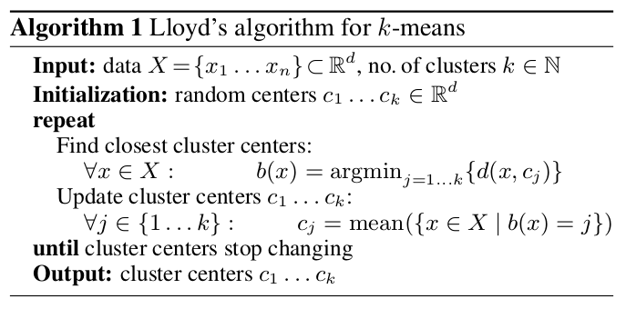
It is easy to show that the above algorithm indeed decreases the $k$-means cost function in each step, so that in the end one obtains a “good” clustering according to the above objective. Note that the algorithm will not guarantee to obtain the global optimum due to the non-convexity of the problem. Instead we will only converge to a local minimum of the above function, but in practice these local optima are usually good enough. In fact, the quality of the obtained results has made $k$-means clustering one of the most widely used clustering techniques.

Among the reasons for the popularity of Lloyd’s algorithm is its simplicity, geometric intuition as well as its experimentally proven ability to find meaningful clusters. However, when applied to a large amount of data in high dimensions, it becomes incredibly slow. Why is this the case?

Main computational bottleneck: distance calculations

Let’s have a closer look at the two steps in the $k$-means algorithm. In the cluster update step, one needs to compute the mean of the points in each cluster. We have to look at each point once, which implies that this step has complexity $O(nd)$ where $n$ is the number of points and $d$ the dimension. In an efficient implementation, this can be done really fast by doing incremental updates of the means and using the fact that some clusters do not change between iterations.

On the other hand, the cluster assignment step is much more time-consuming. In a naive implementation of the algorithm, one computes the Euclidean distances between all points and all cluster centers in order to find the closest one in each iteration. This is of complexity $O(nkd)$, where $k$ is the number of clusters. For large sample sizes, this becomes the main bottleneck and prevents the algorithm from being scalable to large datasets and high dimensions.

Several authors proposed different variants of $k$-means with the goal of reducing the amount of required distance computations. We refer to the discussion in our paper for an overview about previous work on speeding up $k$-means. One recurring theme in the optimizations of $k$-means (see for example the work by Elkan, Hamerly, Drake & Hamerly and recently Ding et al.) is that the techniques rely on the computation of lower bounds on the distances to the cluster centers which are then used to eliminate the actual computation of the distance.

Note that our goal is to have an exact method in the sense that one can guarantee that it achieves the same result as Lloyd’s algorithm, given the same initialization. In a different line of research, several authors developed methods to compute approximate solutions of the $k$-means problem very efficiently, for example based on random subsampling and approximate nearest neighbour search. While these approximate techniques have been shown to lead to significant speed-ups compared to standard $k$-means, they cannot guarantee to obtain the same results as Lloyd’s algorithm which has been shown to work in practice.

Skipping distance calculations by using lower bounds

Above we observed that the computation of Euclidean distances between points $x\in \R^d$ and cluster centers $c\in \R^d$ becomes the main bottleneck when dealing with large dimensions $d$. We now discuss the general idea of how to utilize lower bounds to limit the number of unnecessary distance calculations.

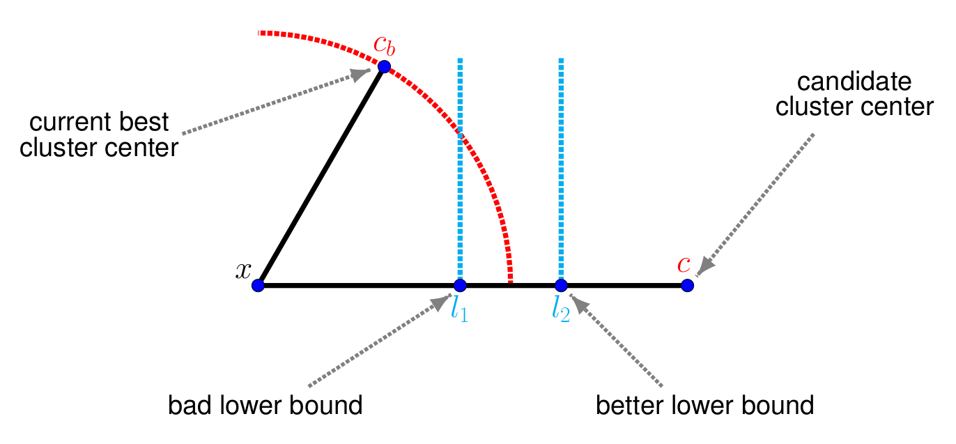
Assume we are in the middle of the assignment step. For a given point $x \in \R^d$, we have already looked at a couple of candidate clusters and the currently best cluster center is $c_b\in \R^d$. The task is now to decide whether a different cluster center $c \in \R^d$ is closer to $x$ than $c_b$. Normally one would need to perform a full distance calculation of $d(x,c)$. However, if a lower bound $l_2=\lb(x,c)$ on the distance $d(x,c)$ is known, and it holds that $l_2 \geq d(x,c_b)$, then clearly also $d(x,c)$ has to be larger than $d(x,c_b)$. Thus one can conclude that $c$ cannot be the closest cluster center and the computation of the distance $d(x,c)$ can be skipped.

In order for this technique to work efficiently, the lower bound $\lb(x,c)$ needs to fulfill two conditions: on one hand, it needs to be as tight as possible, in order to maximize the chance that indeed $\lb(x,c) \geq d(x,c_b)$. The above illustration shows an example where this is not the case: the bound $l_1$ is not helpful to decide whether the cluster $c$ can be skipped or not, and in this case, still a full distance calculation needs to be done.

On the other hand, the lower bound needs to be efficiently computable, in order to achieve the desired overall improvement in runtime and memory requirement. In practice, one usually observes a certain trade-off between a bound which is easy to compute but quite loose, and a very tight bound which leads to many skipped distance calculations but is more costly. We will now discuss several different attempts to compute lower bounds on the Euclidean distance.

First attempt: Cauchy-Schwarz inequality

The practicality of the lower-bound based methods hinges on the tightness of the bounds as well as the efficiency in which they can be computed. For this reason we will now further investigate how to obtain lower bounds which satisfy these properties. We start by noting that the squared Euclidean distance can be decomposed into

Our first approach is to use the Cauchy-Schwarz inequality, which states that for all $x,c\in\R^d$,

It is now straightforward to combine these results and obtain the simple lower bound

By rewriting the bound as $\lb\supC(x,c) = \abs{ \norm{x}_2- \norm{c}_2}$, we see that it has a nice geometric interpretation: it is the difference between the length of the largest and smallest of the two vectors $x$ and $c$. With the reasoning given in the previous section, we could use this bound to skip redundant distance calculations: all $c \in C$ with $\lb\supC(x,c) \geq d(x,c_b)$ cannot be closer to $x$ than $c_b$ and can be skipped in the distance calculation step.

If the values of $\norm{x}_2$ and $\norm{c}_2$ are precomputed, then the bound can be obtained very efficiently. However, while it can already lead to some avoided computations it is too loose to be effective in general. To see this, consider the following simple example: Suppose $x \in \R^{d}$ is a point with $x_1 = 1$ and zero else, and $c \in \R^{d}$ is a second point only consisting of ones. Then the dot product $\inner{x, c}$ between these two points is equal to $1$. The approximation $\norm{ x }_2 \norm{ c }_2$ however is $\sqrt{d}$, which can be considerably higher, thus leading to a loose lower bound.

Second attempt: Hölder’s inequality

The next idea is to generalize the above bound by replacing the Cauchy-Schwarz inequality by Hölder’s inequality, which states that for any $1 \leq p,q \leq \infty$ with $\tfrac{1}{p} + \tfrac{1}{q} = 1$, it holds that

where $\norm{x}_p$ denotes the $l^p$-norm of $x \in \R^d$, defined for $p\geq1$ as $\norm{x}_p:= \left(\sum_{i=1}^n \abs{x_i}^p\right)^{1/p }$. Moreover, we use the usual definition $\norm{x}_{\infty} := \lim_{p \rightarrow \infty} \norm{x}_p = \max_{i} \abs{x_i}$. For $p=2$, one obtains the standard Euclidean norm. Analogously to the Cauchy-Schwarz case, one can combine this with the definition of the Euclidean distance, leading to

Note that while in the Cauchy-Schwarz case ($p=q=2$), the right side is guaranteed to be non-negative, this is not true in general. Thus one needs to add an additional $\max$ term before taking the square root. The lower bound on the Euclidean distance then becomes

Particularly interesting are the limit cases $p \rightarrow 1$ and $q \rightarrow 1$, where the inner product becomes upper bounded by $\norm{ x }_1 \max_i \abs{c_i}$ and $\max_i \abs{x_i}\norm{ c }_1$, respectively. As in the case of the Cauchy-Schwarz inequality, the bounds can be easily computed. Unfortunately, while they seem to be tighter in some cases, they are not generally better than the standard Cauchy-Schwarz ones and still often too loose. Thus, we need to find a way to tighten the lower bounds.

Third attempt: Tightened Hölder’s inequality

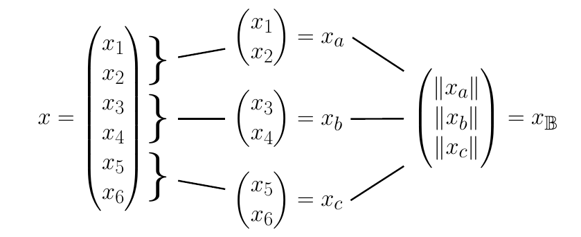
Before discussing how to obtain tighter lower bounds, we will first describe the blockification process which will play an essential role. The main idea is that a point $x \in \R^{d}$ can be subdivided into $b$ blocks $x_{(1)} \dots x_{(b)}$ of sizes $\ge 1$ by splitting along its dimensions, i.e. one has $x_{(1)}=(x_{1}\dots x_{l_1})$, $x_{(2)}=(x_{l_1+1}\dots x_{l_2})$ and so on, where $0 = l_0 < \ldots < l_b=d$ is an increasing sequence of indices. Then one can construct a vector $x_{\Bp} \in \R^{b}$ with $b \le d$ by calculating the $p$-norm of every block and setting $(x_{\Bp})_i := \norm{x\subi}_p$. We will refer to the vector $x_{\Bp}$ as block vector. The blockification process is equal to the compression technique by Low & Zheng applied to a one-dimensional matrix. Below is an example for the case $d=6$ and $b=3$.

The above block vector can now be used to obtain a tightened Hölder’s inequality. Namely, for $x,c\in \R^d$, block vectors $x_{\Bp}, c_{\Bq} \in \R^b$, and $p$, $q$ as above, it is easy to show that

For $p=q=2$ one obtains the following tightened Cauchy-Schwarz inequality as special case:

Different values of $b$ lead to different intuitive solutions. Let’s consider the two extreme cases: if we set $b = d$ (the number of blocks is equal to the number of dimensions), then $x_{\Bp} = x$ and $\inner{ x,c } = \inner{ x_{\Bp},c_{\Bq} }$ and hence the left inequality is tight. On the other hand, if $b = 1$ (only one block) then $\inner{ x_{\Bp},c_{\Bq}} = \norm{ x }_p \norm{ c }_q$, and we obtain Hölder’s inequality. With the option to choose $b$ the quality of the dot product approximation can be controlled.

Note that the above approximation is especially useful in the case of sparse datasets. To see this, observe that in the case where $x\subi = 0$ for some block $i$ (or analogously $c\subi = 0$), we have $0 = \inner{x\subi, c\subi} \leq \norm{x\subi}_p \norm{c\subi}_q=0$, which means that in this case, the corresponding part of the inner product $\inner{x, c}$ gets approximated exactly. However, the corresponding part $c\subi\neq 0$ (or analogously $x\subi\neq 0$) would still contribute to $\norm{x}_p \norm{c}_q$ while it has no influence on $\norm{x\subi}_p \norm{c\subi}_q$. For large sparse datasets, typically this case occurs very frequently.

The above tightened versions of Hölder’s and Cauchy-Schwarz inequality can be used to derive the tightened lower bounds on the Euclidean distance: Namely, given $x,c\in \R^d$, block vectors $x_{\Bp}, c_{\Bq} \in \R^b$, and $p$, $q$ as above, a lower bound on $d(x,c)$ is given by

As a special case, one again obtains for $p=q=2$ the tightened lower bound

For the choice of $b=1$, the above lower bounds coincide with the ones obtained when using the standard Hölder’s or Cauchy-Schwarz inequality, while for $b>1$ we obtain tighter bounds than the standard ones. In the case $b=d$ the bounds coincide with the Euclidean distance. To further illustrate the improved approximation, let us again consider our example from before where the dot product of the vectors $x$ and $c$ was $1$. Consider the case $p=2$ and suppose $x$ and $c$ are split into $b$ blocks of equal sizes. The approximation with block vectors then is $\inner{ x_{\B2},c_{\B2} } = \sqrt{d/b}$ which can be considerably closer to $1$ in this ideal example.

Regarding the time needed to compute the bounds, note that the block vectors do not need to be constructed in each step. The block vectors for each point can be computed in a single pass at the beginning of the algorithm. This implies that we only need to compute the block vectors for the cluster centers in each iteration. With the block vectors precomputed, the evaluation of the above lower bounds then is very efficient. However, it is clear that for a too high value of $b$ the precomputation and storing of the block vectors becomes the main bottleneck and hence obtaining the lower bound can get expensive.

We will further investigate the trade-off between achieving a good approximation of the Euclidean distance and fast computation of the bounds for different choices of $b$ later in this post. Before that let’s first talk about how to incorporate the above techniques into $k$-means.

Block vector optimized $k$-means

In the following we show how the proposed technique is used to derive optimized variants of standard $k$-means. For simplicity of notation, we restrict ourselves to the case $p=2$ and omit the subscripts for $p$ in the notation for the block vectors, norms, etc. However, all results also carry over to the general case. The following algorithm uses the lower bounds obtained in the previous section through our blockification strategy.

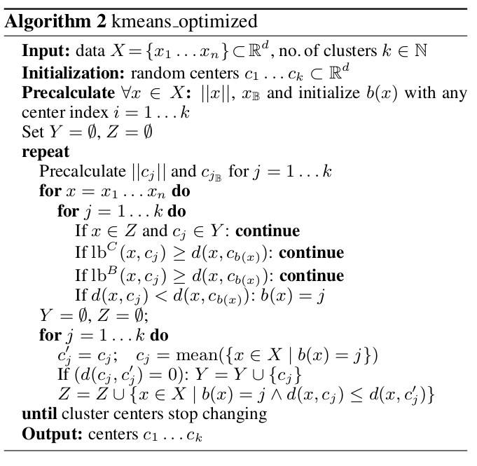
At the beginning of the above algorithm, a precalculation step is performed where all data required to compute the lower bounds are computed for all points $x$. At the start of every iteration the same is done for the cluster centers $c_1 \dots c_k$. Then, in the cluster assignment step, while iterating through the centers to find the closest one for every $x$, the lower bounds are evaluated in order of increasing cost, starting with the cheapest but loosest bound. Only if no lower bound condition was met, $d(x,c)$ has to be calculated in order to decide whether $c$ becomes the new closest center, indexed by $b(x)$. After updating $b(x)$ for all $x$, the clusters are shifted analogously to standard $k$-means.

In the initial phase of the algorithm, the cost of calculating the lower bounds between every point and center is compensated by the speed-up achieved due to the reduced amount of distance calculations. However, near convergence, when few clusters are shifting, the additional cost of obtaining the lower bounds outweighs its gain. Thus we use the following additional optimization (see e.g. here or here): let $c'$ be the closest cluster center to $x$ before shifting, and $c$ the center after shifting. If $d(x, c) \le d(x,c')$, then all cluster centers $c_1 \dots c_k$ which did not shift in the last iteration cannot be closer to $x$ than $c$. Thus, in the above algorithm we maintain two sets $Y$ and $Z$: the set $Y$ contains all cluster centers which did not shift in the last iteration, while the set $Z$ contains all points $x$ with $d(x, c) \le d(x,c')$.

Recently, Ding et al. proposed an enhanced version of $k$-means called Yinyang $k$-means. In their paper it was shown that an initial grouping of the cluster centers can be used to obtain an efficient filtering mechanism to avoid redundant distance calculations. Our blockification strategy discussed above utilizes a grouping of the input dimensions and can thus be seen as complementary to the one by Ding et al. In order to combine the strengths of both methods, we also incorporated our block vectors into their algorithm, yielding a method referred to as Fast Yinyang. An in-depth discussion of our optimization of Yinyang $k$-means would be outside the scope of this post, thus we refer to our paper for further technical details.

Determining the block vector size

The question remains what is a good value for the number of blocks used in the blockification technique described above. To answer this question, an experiment with the block vector optimized $k$-means was conducted, where we observed the clustering duration for various block vector sizes for several datasets downloaded from the libsvm homepage. Below we show the clustering duration for the datasets usps and sector for a static $k$ of $1000$.

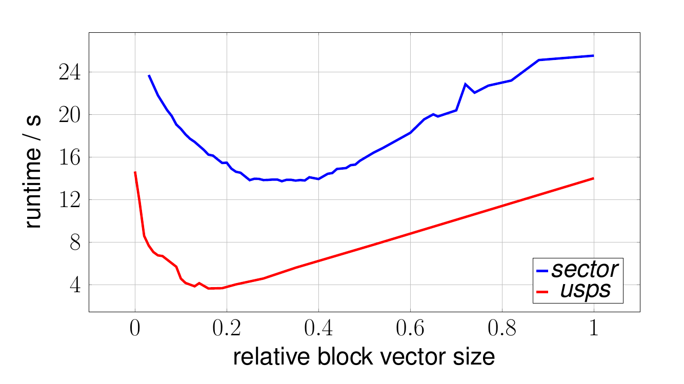
Note that instead of reporting absolute block vector sizes in the x-axis, we use the relative number of non-zero elements in the block vectors, which is more appropriate in a sparse setting. To be more precise, we use the ratio $\frac{\annz(X_\B)}{\annz(X)}$, where for a set of samples $X=\{x_1 \dots x_n\}$, the notation $\annz(X) := \tfrac{1}{n} \sum_{i=1}^n \nnz(x_i)$ denotes the average number of non-zero elements, with $\nnz(x)$ denoting the number of non-zeros elements of $x$.

In the plot one clearly observes the trade-off controlled by the parameter $b$: if one increases the value of $b$ (more blocks), the bound becomes tighter but also the time to compute it increases. In the limit case (right side of the plot) the bound is tight but this does not help since it agrees with the actual distance. On the other hand, if one chooses $b$ too small (few blocks), the bound becomes too loose and does not often lead to skipped distance calculations. In this case, computing the lower bound increases the total time since one needs to compute the actual distance anyway (note that we plot the total time including the possible distance calculation).

The optimal trade-off is obviously achieved somewhere inbetween those two extreme cases, as can be observed for both datasets. Of course the exact value of the optimal parameter of $b$ is dataset dependent. Typically a value $b$ leading to $0.15\,\annz(X) \le \annz(X_\B) \le 0.4\,\annz(X)$ results in a short clustering duration.

Based on the results from this experiment, in the following the size of the block vectors is chosen in such a way that $\annz(X_\B) \approx 0.3\,\annz(X)$. This is achieved by starting with a static initial block size, and iteratively reducing the block size until $\annz(X_B) \le 0.3\, \annz(X)$ holds. In our experiments, this iterative procedure typically needs around 3-4 steps until the condition is met.

Memory consumption

In general other lower bound based techniques such as Elkans’s $k$-means or Yinyang $k$-means already save a lot of distance calculations. However, with increasing $k$ the memory consumption and computational cost required to maintain the necessary data structures grow quadratically for Elkans’s $k$-means, making it slow for large numbers of clusters. In the case of Yinyang $k$-means, storing the groups requires $\frac{k}{10} \cdot n$ memory.

On the other hand, creating the block vectors in memory is very cheap compared to computing even one iteration of $k$-means. If $r := \annz(X) \cdot n$ is the memory needed to store the input matrix $X$ (sparse), then the block vectors $X_\B$ require about $0.3 r$ memory. The worst case memory consumption due to block vectors is therefore $0.3r$ for $X_\B$ plus an additional $0.3r$ for the storage of the cluster center block vectors. This worst case is only reached in the extreme case where every sample is a cluster.

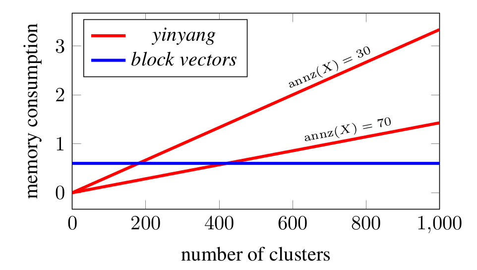
We see that when increasing $k$, Yinyang exceeds the constant worst case memory consumption of the block vectors. Storing the block vectors gets cheaper (relative to total memory consumption) with increasing sparsity of $X$ while Yinyang does not profit from a higher sparsity.

Dependency on number of clusters

As discussed above, the nature of how block vectors are constructed makes them very useful especially for sparse data. In a sparse setting, since the cluster centers are computed as the mean of the points in the corresponding cluster, they tend to become more sparse with increasing $k$. At the same time the evaluation of the dot product between the samples and between the block vectors gets cheaper. Additionally, for sparser data, the approximation of the distances through block vectors gets more accurate.

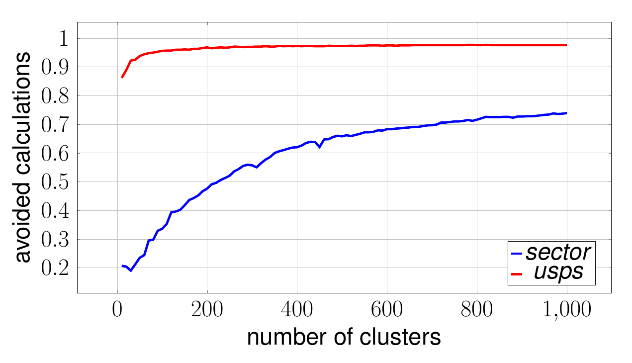
The above plot shows the result of an experiment conducted using our optimized k-means for the sector and the usps dataset. Several runs where performed where the block vector size was fixed and the number of clusters $k$ was varied between $2$ and $1000$. The $y$-axis denotes the number of avoided distance calculations, which indicates how good the lower bound $\lb\supB(x,c)$ approximates the actual distance $d(x,c)$. It can be observed that for both datasets the percentage of avoided distance calculations increases with the number of clusters $k$.

Speed-up over standard $k$-means

Finally we show empirical evaluations of the total runtime of the standard and our optimized versions of $k$-means and Yinyang on several datasets (more results can be found in the paper). Prior to experimentation, the datasets have been scaled to the range between $0$ and $1$. The plots below display the relative speed-up over a non-optimized standard $k$-means.

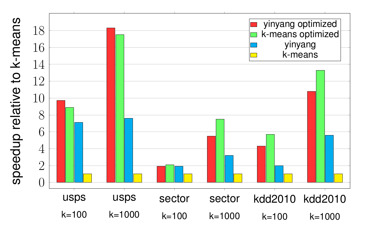
The same initial cluster centers are chosen for all methods. As a consequence, exactly the same clustering is generated after every iteration. The reported results include the time to create the initial block vectors for $X$ as well as the block vectors for the clusters. One observes that while Yinyang already achieves a big speed-up compared to standard $k$-means, it is often significantly outperformed by our optimized variants especially for large number of clusters.

Conclusion

In this post we demonstrated a simple and efficient technique to speed-up $k$-means, particularly suited to the case where the aim is to cluster large amounts of high-dimensional sparse data into many clusters. The main technical tool was a tightened Hölder’s inequality obtained by using a concept referred to as blockification, which lead to better lower bound approximations of the Euclidean distances. While in the above work we considered only a blockification strategy based on evenly-spaced blocks, one could imagine that a smarter blocking scheme could lead to even tighter bounds and thus even greater speed-ups. Thus there is ample opportunity for further research. Moreover, the proposed technique is not only limited to $k$-means clustering but could be helpful for a wide range of other distance-based techniques in machine learning.

Thomas Bottesch, Thomas Bühler, Markus Kächele. Speeding up k-means by approximating Euclidean distances via blockvectors. ICML 2016.